By Dr. Don J. Wood and Dr. Srinivasa Lingireddy
Back in the 1960’s pipe system transient analysis code using a technique developed by Dr. Wood was written to handle propellant flow transients for NASA. This technique, initially referred as the Wave Plan Method, was further developed and around 1984 the first commercial software (SURGE1) was released for general use. Since then several thousand software packages have been supplied to engineers worldwide and this software has been applied extensively, undergone numerous QA procedures (nuclear facilities) and, in general, been exhaustively tested and verified.
It has been suggested that the Wave Characteristic Method (WCM), a.k.a. Wave Plan Method, is less accurate than the original Method of Characteristics (MOC) for transient pipe flow analysis. This is a totally false representation. The reality is that the MOC is a very inefficient technique for pipeline transient analysis. Handling larger piping systems will often be impossible using the MOC or will take hours compared to minutes to attain a solution.
Accuracy of Calculations
Below are three examples of transient analysis solutions using the Method of Characteristics (MOC) and the Wave Characteristic Method (WCM).
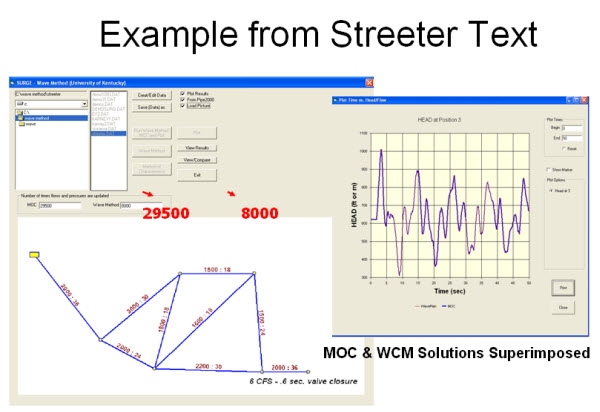
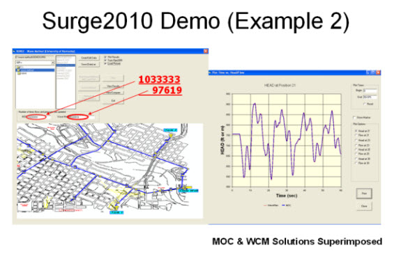
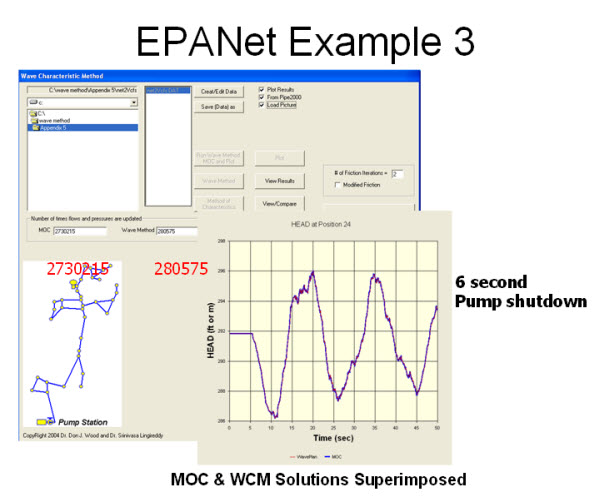
The most distinguishing characteristics of these comparisons are that they are virtually identical even though the wave forms are quite irregular. Is this surprising? NO! This is exactly what we expect because both techniques accurately solve the complex partial differential transient flow momentum and continuity equations. Any differences would be most disturbing and unacceptable.
These results are detailed in the reference shown below.
| Example 1 is an example of a valve closure from Streeter & Wylie’s classic Fluid Transients textbook. Note the comparisons in the MOC and WCM are superimposed on one another in both the upper and lower pictures. The upper comparison uses a MOC computer analysis developed by Dr. Lingireddy (yes- we are totally familiar with MOC technology). The lower comparison uses a MOC computer analysis developed by Dr. Bryan Karney of the University of Toronto using his widely used TRANSM software. |
 |
 |
| Example 2 is an example of a rapid pump shutdown in a more complex network. Again the results from the MOC and WCM analyses are superimposed. |
|
| Example 3 is from the EPANET Users guide and shows two sets of comparisons. |
|
Efficiency of the Calculations: The really significant characteristic of the solutions is that the WCM approach normally requires orders of magnitude fewer calculations and orders of magnitude less computer memory to attain the same accurate solution. For smaller piping systems with only a few pipes or relatively short pipes (such as these examples) this is not a huge issue. But for larger systems such as a typical water distribution system the MOC may be unable to handle the massive amount of storage and calculations required. If obtaining a solution is possible the MOC solution may require hours as compared to minutes for the WCM solution.
Make no mistake about it, transient pipe flow analysis requires a tremendous number of calculations. For example to analyze a piping system with wave speeds on the order of 4000 ft/s (say ductile iron) and model the pipe lengths to a tolerance of 10 feet requires a computational time increment of 10/4000 or 2.5 milliseconds or 400 computations per second. A 200 second simulation will require 80,000 computations at each nodal point in the pipe system. The number of nodal points requiring calculations is where the differences between the WCM and the MOC become very pronounced.
The MOC is essentially a finite differencing scheme for solving complex partial differential equations. The scheme requires that computational nodal points be located at equally spaced distances along each pipeline and the distance between these computational nodes is equal to the length tolerance used for the model. If, for example, a pipeline is 2000 feet long, a 10 foot length tolerance would require an interior computational node every 10 feet or 200 interior nodes. For the previous example 80,000 calculations are required for each of the 200 interior nodes in addition to the end nodes. Calculation are made each time increment at a all nodes using the results at all immediately adjacent nodes obtained the previous time increment. In this manner a disturbance initiated at a pump for example will be transmitted to the next adjacent node each time increment. In the 2000 foot long pipe previously discussed it would take 200 time increments for the disturbance to be propagated to the opposite end of the pipe. The interior computational nodes are used primarily for propagating disturbances throughout the piping system.
The WCM basically uses well known properties of pressure waves to avoid the need to use interior computational nodes to transmit disturbances. Pressure waves travel at a constant speed in a pipeline so it is a very simple procedure to determine the nature of the waves impinging at an end node (pump, valve, junction, etc) at any time during a simulation. For example, using the 2000 foot long pipeline discussed above the pressure wave impinging at one end of a 2000 foot long pipeline is the one which left the node at the other end 200 time increments earlier. Applying this logic it is possible to solve the basic momentum and continuity relationships by making calculations only at the end nodes and using the characteristics of pressure waves to bypass the tedious interior calculations. Again, referring to the 200 foot long pipeline we can get the identical solution by keeping tabs on pressure wave movements and making calculations only at the 2 end nodes (using the WCM) as we will get making an additional 200 calculations at the interior computational nodes (using the MOC).
Additional Considerations: Another misleading claim we hear is that an important result may be missed because the WCM does not do the tedious and unnecessary internal calculations. This argument is totally without merit. Internal nodes may be placed at any desired location using the WCM. We strongly feel that a knowledgeable modeler will add internal nodes at high (or low) elevations and any other location that may be of interest or improve the results presentations. This should be their choice. In a typical water distribution system there may be several locations of interest. Certainly no knowledgeable user would add many thousands of internal computational nodes because something may be missed. Consider how ludicrous this approach would be if applied to steady state modeling.
Conclusions: The WCM approach to handling pressure wave action in pipe systems represents a well tested and widely used major advancement in pipe flow transient analysis. Using this technique it is possible to accurately analyze large piping systems and long pipelines. In spite of various claims, there are no legitimate disadvantages to this approach and the computational advantages are HUGE. The authors will be happy to discuss transient analysis with potential clients.