Chapter 1 – Wave Plan Method
Surge Analysis and the Wave Plan Method
Supplementary Material: Example Problems and Solutions
Chapter 1 – Problem 1.23
1.23 Consider a branched pipe network where the valve at the end of mainline is closed. The initial flows and pressure heads are shown on the network schematic below. Assume that all the nodes are at 0 elevation. Track the pressure waves for at least two time steps accounting for pipe frictional resistance.

Solution:
The valve at the end of the branch line closes instantaneously at time 0 generating a pressure wave of 90m. This wave reaches the three-pipe junction node in one Δt.

However, the pressure wave also is altered by the frictional resistance in Pipe-1 (see section 1.7 and other referenced figures and equations in the book “Surge Analysis and the Wave Plan Method“). Eq. 1.64 can be used (along with Figure 1.27 for the appropriate sign convention) to compute the flowrate in Pipe-1 after the wave action at the friction orifice. The notation used in Figure 1.27 can be applied to Pipe-1 as shown in the following.
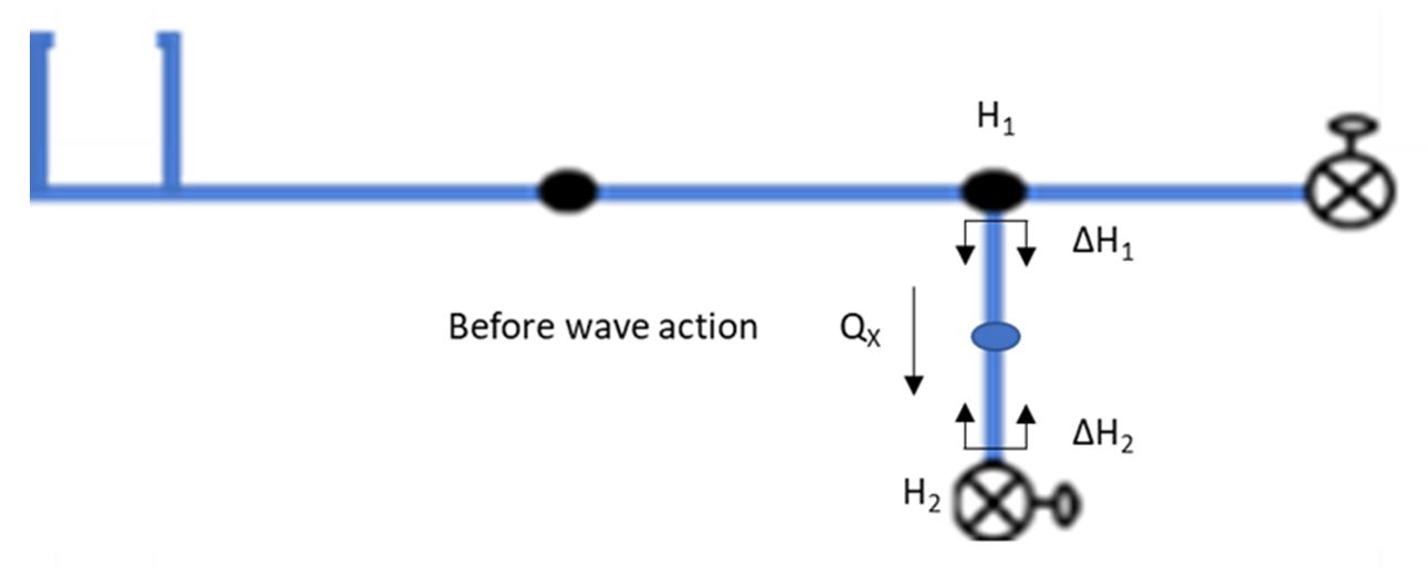

Pipe-1: In the above schematic, QX = 1.0 m3/s, H1 = 101m, H2 = 100m, ΔH1 = 0m, ΔH2 = 90m. The resistance associated with Pipe-1 is K = (H1 – H2)/QX2= 1 (Eq. 1.44). The elastic factor F for Pipe-1 is 100. Substituting these values in Eq. 1.64:
K + 2FQY – (H1 – H2 + 2∆H1 -2∆H2 + 2FQX) = 0 results in the following quadratic equation for QY.
+ 200 QY – 21 = 0
By solving this quadratic equation, QY = +0.10495 m3/s.
Using Eqs. 1.58 through 1.61: ΔHR = +89.5m, ΔHT = +0.5m, H3 = 190.5m, and H4 = 100.5m. Pressure waves after wave action at the friction orifice and a subsequent junction analysis are shown in the following.

Pipe-2. The pressure wave of +59.66m originating at the junction reaches the valve end of the pipe in one Δt at which point wave is reflected from the valve and travels back towards the junction. The associated reflected and transmitted pressure waves are computed using Eq. 1.64. Substituting QX = 0.0 m3/s, H1 = 101m, H2 = 101m, ΔH1 = 59.66m, ΔH2 = 0m, and F = 100 in Eq. 1.64 results in the following quadratic equation.
+ 200 QY – 119.32 = 0
By solving the above quadratic equation, QY = +0.595 m3/s. Using Eqs. 1.58 and 1.60: ΔHR = +0.16m and ΔHT = +59.5m for Pipe-2.
Pipe-3. Similarly, the reflected and transmitted pressure waves for Pipe-3 are: ΔHR = +59.2m and ΔHT = +0.46m, and for Pipe-1 are: ΔHR = -45.46m and ΔHT = +37.125m

Summary of revisions to this page:
Date/Revision